NumPy 与 Pandas [课程]
NumPy and Pandas [Course]

Udacity course link: https://www.udacity.com/course/intro-to-data-analysis--ud170
NumPy arrays
Be careful when operating NumPy arrays.
import numpy as np
a = np.array([1,2,3,4])
b = a
a += np.array([1,1,1,1])   # In-place, use `b = a.copy()` to avoid
print b   # [2,3,4,5]

import numpy as np
a = np.array([1,2,3,4])
b = a
a = a + np.array([1,1,1,1])   # Not in-place
print b   # [1,2,3,4]

import numpy as np
a = np.array([1,2,3,4])
slice = a[:3]
slice[0] = 100   # Change even in slicing! Diff from list
print a   # [100,2,3,4]
Pandas series
Pandas series is similar to NumPy array, but with extra functionality.
import pandas as pd
tmp = pd.Series([1,3,2,4],index=['a','c','b','d'])
print tmp
# Output:
a    1
c    3
b    2
d    4
dtype: int64

print tmp.loc['c']   # 3

print tmp.idxmax()   # d

# When adding two Pandas Series, only same indexes will be added,
# otherwise NaN
s1 = pd.Series([1, 2, 3, 4], index=['a', 'b', 'c', 'd'])
s2 = pd.Series([10, 20, 30, 40], index=['c', 'd', 'e', 'f'])
print s1 + s2

s3 = s1 + s2
s3.dropna(inplace=True)   # Drop NaN
# s3.fillna(0, inplace=True)   # Fill NaN with 0

s = pd.Series([1, 2, 3, 4, 5])
def add_one(x):
    return x + 1
print s.apply(add_one)   # apply(): vectorized operation
NumPy array: 2D
import numpy as np

# Subway ridership for 5 stations on 10 different days
ridership = np.array([
    [   0,    0,    2,    5,    0],
    [1478, 3877, 3674, 2328, 2539],
    [1613, 4088, 3991, 6461, 2691],
    [1560, 3392, 3826, 4787, 2613],
    [1608, 4802, 3932, 4477, 2705],
    [1576, 3933, 3909, 4979, 2685],
    [  95,  229,  255,  496,  201],
    [   2,    0,    1,   27,    0],
    [1438, 3785, 3589, 4174, 2215],
    [1342, 4043, 4009, 4665, 3033]
])

# Change False to True for each block of code to see what it does

# Accessing elements
print ridership[1, 3]
print ridership[1:3, 3:5]
print ridership[1, :]

# Vectorized operations on rows or columns
print ridership[0, :] + ridership[1, :]
print ridership[:, 0] + ridership[:, 1]

# Vectorized operations on entire arrays
a = np.array([[1, 2, 3], [4, 5, 6], [7, 8, 9]])
b = np.array([[1, 1, 1], [2, 2, 2], [3, 3, 3]])
print a + b
NumPy axis
import numpy as np

a = np.array([
    [1, 2, 3],
    [4, 5, 6],
    [7, 8, 9]
])

print a.sum()   # 45
print a.sum(axis=0)   # [12 15 18]
print a.sum(axis=1)   # [ 6 15 24]
Accessing data from a Pandas DataFrame
import pandas as pd

# Subway ridership for 5 stations on 10 different days
ridership_df = pd.DataFrame(
    data=[[   0,    0,    2,    5,    0],
          [1478, 3877, 3674, 2328, 2539],
          [1613, 4088, 3991, 6461, 2691],
          [1560, 3392, 3826, 4787, 2613],
          [1608, 4802, 3932, 4477, 2705],
          [1576, 3933, 3909, 4979, 2685],
          [  95,  229,  255,  496,  201],
          [   2,    0,    1,   27,    0],
          [1438, 3785, 3589, 4174, 2215],
          [1342, 4043, 4009, 4665, 3033]],
    index=['05-01-11', '05-02-11', '05-03-11', '05-04-11', '05-05-11',
           '05-06-11', '05-07-11', '05-08-11', '05-09-11', '05-10-11'],
    columns=['R003', 'R004', 'R005', 'R006', 'R007']
)

# Change False to True for each block of code to see what it does

# DataFrame creation
# You can create a DataFrame out of a dictionary mapping column names to values
df_1 = pd.DataFrame({'A': [0, 1, 2], 'B': [3, 4, 5]})
print df_1
# You can also use a list of lists or a 2D NumPy array
df_2 = pd.DataFrame([[0, 1, 2], [3, 4, 5]], columns=['A', 'B', 'C'])
print df_2

# Accessing elements
print ridership_df.iloc[0]
print ridership_df.loc['05-05-11']
print ridership_df['R003']
print ridership_df.iloc[1, 3]

# Accessing multiple rows
print ridership_df.iloc[1:4]

# Accessing multiple columns
print ridership_df[['R003', 'R005']]

# Pandas axis
df = pd.DataFrame({'A': [0, 1, 2], 'B': [3, 4, 5]})
print df.sum()
print df.sum(axis=1)
print df.values.sum()
# Instead of axis=0/1, can use axis='index'/'columns'
Read in Pandas DataFrame
import pandas as pd

filename = '/datasets/ud170/subway/nyc_subway_weather.csv'
subway_df = pd.read_csv(filename)
DataFrame vectorized operations
import pandas as pd

# Adding DataFrames with the column names
df1 = pd.DataFrame({'a': [1, 2, 3], 'b': [4, 5, 6], 'c': [7, 8, 9]})
df2 = pd.DataFrame({'a': [10, 20, 30], 'b': [40, 50, 60], 'c': [70, 80, 90]})
print df1 + df2

    a   b   c
0  11  44  77
1  22  55  88
2  33  66  99

# Adding DataFrames with overlapping column names
df1 = pd.DataFrame({'a': [1, 2, 3], 'b': [4, 5, 6], 'c': [7, 8, 9]})
df2 = pd.DataFrame({'d': [10, 20, 30], 'c': [40, 50, 60], 'b': [70, 80, 90]})
print df1 + df2

    a   b   c   d
0 NaN  74  47 NaN
1 NaN  85  58 NaN
2 NaN  96  69 NaN

# Adding DataFrames with overlapping row indexes
df1 = pd.DataFrame({'a': [1, 2, 3], 'b': [4, 5, 6], 'c': [7, 8, 9]},
                   index=['row1', 'row2', 'row3'])
df2 = pd.DataFrame({'a': [10, 20, 30], 'b': [40, 50, 60], 'c': [70, 80, 90]},
                   index=['row4', 'row3', 'row2'])
print df1 + df2

         a     b     c
row1   NaN   NaN   NaN
row2  32.0  65.0  98.0
row3  23.0  56.0  89.0
row4   NaN   NaN   NaN

# DataFrame applymap(): operate on one element a time
df = pd.DataFrame({
    'a': [1, 2, 3],
    'b': [10, 20, 30],
    'c': [5, 10, 15]
})

def add_one(x):
    return x + 1

print df.applymap(add_one)

   a   b   c
0  2  11   6
1  3  21  11
2  4  31  16

# DataFrame apply(): operate on one column a time

grades_df = pd.DataFrame(
    data={'exam1': [43, 81, 78, 75, 89, 70, 91, 65, 98, 87],
          'exam2': [24, 63, 56, 56, 67, 51, 79, 46, 72, 60]},
    index=['Andre', 'Barry', 'Chris', 'Dan', 'Emilio',
           'Fred', 'Greta', 'Humbert', 'Ivan', 'James']
)

def convert_grades_curve(exam_grades):
    # Pandas has a bult-in function that will perform this calculation
    # This will give the bottom 0% to 10% of students the grade 'F',
    # 10% to 20% the grade 'D', and so on. You can read more about
    # the qcut() function here:
    # http://pandas.pydata.org/pandas-docs/stable/generated/pandas.qcut.html
    return pd.qcut(exam_grades,
                   [0, 0.1, 0.2, 0.5, 0.8, 1],
                   labels=['F', 'D', 'C', 'B', 'A'])

# qcut() operates on a list, array, or Series. This is the
# result of running the function on a single column of the
# DataFrame.
print convert_grades_curve(grades_df['exam1'])

Andre      F
Barry      B
Chris      C
Dan        C
Emilio     B
Fred       C
Greta      A
Humbert    D
Ivan       A
James      B
Name: exam1, dtype: category
Categories (5, object): [F < D < C < B < A]

# qcut() does not work on DataFrames, but we can use apply()
# to call the function on each column separately
print grades_df.apply(convert_grades_curve)

        exam1 exam2
Andre       F     F
Barry       B     B
Chris       C     C
Dan         C     C
Emilio      B     B
Fred        C     C
Greta       A     A
Humbert     D     D
Ivan        A     A
James       B     B
Adding a DataFrame to a Series:
import pandas as pd

# Adding a Series to a square DataFrame
s = pd.Series([1, 2, 3, 4])
df = pd.DataFrame({
    0: [10, 20, 30, 40],
    1: [50, 60, 70, 80],
    2: [90, 100, 110, 120],
    3: [130, 140, 150, 160]
})

print df
print '' # Create a blank line between outputs
print df + s

    0   1    2    3
0  10  50   90  130
1  20  60  100  140
2  30  70  110  150
3  40  80  120  160

    0   1    2    3
0  11  52   93  134
1  21  62  103  144
2  31  72  113  154
3  41  82  123  164

# Adding a Series to a one-row DataFrame
s = pd.Series([1, 2, 3, 4])
df = pd.DataFrame({0: [10], 1: [20], 2: [30], 3: [40]})

print df
print '' # Create a blank line between outputs
print df + s

# Adding a Series to a one-column DataFrame
s = pd.Series([1, 2, 3, 4])
df = pd.DataFrame({0: [10, 20, 30, 40]})

print df
print '' # Create a blank line between outputs
print df + s

    0
0  10
1  20
2  30
3  40

    0   1   2   3
0  11 NaN NaN NaN
1  21 NaN NaN NaN
2  31 NaN NaN NaN
3  41 NaN NaN NaN

# Adding when DataFrame column names match Series index
s = pd.Series([1, 2, 3, 4], index=['a', 'b', 'c', 'd'])
df = pd.DataFrame({
    'a': [10, 20, 30, 40],
    'b': [50, 60, 70, 80],
    'c': [90, 100, 110, 120],
    'd': [130, 140, 150, 160]
})

print df
print '' # Create a blank line between outputs
print df + s

    a   b    c    d
0  10  50   90  130
1  20  60  100  140
2  30  70  110  150
3  40  80  120  160

    a   b    c    d
0  11  52   93  134
1  21  62  103  144
2  31  72  113  154
3  41  82  123  164

# Adding when DataFrame column names don't match Series index
s = pd.Series([1, 2, 3, 4])
df = pd.DataFrame({
    'a': [10, 20, 30, 40],
    'b': [50, 60, 70, 80],
    'c': [90, 100, 110, 120],
    'd': [130, 140, 150, 160]
})

print df
print '' # Create a blank line between outputs
print df + s

    a   b    c    d
0  10  50   90  130
1  20  60  100  140
2  30  70  110  150
3  40  80  120  160

    0   1   2   3   a   b   c   d
0 NaN NaN NaN NaN NaN NaN NaN NaN
1 NaN NaN NaN NaN NaN NaN NaN NaN
2 NaN NaN NaN NaN NaN NaN NaN NaN
3 NaN NaN NaN NaN NaN NaN NaN NaN

# Adding using +
s = pd.Series([1, 2, 3, 4])
df = pd.DataFrame({
    0: [10, 20, 30, 40],
    1: [50, 60, 70, 80],
    2: [90, 100, 110, 120],
    3: [130, 140, 150, 160]
})

print df
print '' # Create a blank line between outputs
print df + s

    0   1    2    3
0  10  50   90  130
1  20  60  100  140
2  30  70  110  150
3  40  80  120  160

    0   1    2    3
0  11  52   93  134
1  21  62  103  144
2  31  72  113  154
3  41  82  123  164

# Adding with axis='index'
print df.add(s, axis='index')
# The functions sub(), mul(), and div() work similarly to add()

    0   1    2    3
0  11  51   91  131
1  22  62  102  142
2  33  73  113  153
3  44  84  124  164

# Adding with axis='columns'
print df.add(s, axis='columns')
# The functions sub(), mul(), and div() work similarly to add()

    0   1    2    3
0  11  52   93  134
1  21  62  103  144
2  31  72  113  154
3  41  82  123  164
Pandas groupby()
import matplotlib.pyplot as plt
import numpy as np
import pandas as pd
import seaborn as sns

values = np.array([1, 3, 2, 4, 1, 6, 4])
example_df = pd.DataFrame({
    'value': values,
    'even': values % 2 == 0,
    'above_three': values > 3
}, index=['a', 'b', 'c', 'd', 'e', 'f', 'g'])

# Examine DataFrame
print example_df

  above_three   even  value
a       False  False      1
b       False  False      3
c       False   True      2
d        True   True      4
e       False  False      1
f        True   True      6
g        True   True      4

# Examine groups
grouped_data = example_df.groupby('even')
# The groups attribute is a dictionary mapping keys to lists of row indexes
print grouped_data.groups

{False: Index([u'a', u'b', u'e'], dtype='object'),
 True: Index([u'c', u'd', u'f', u'g'], dtype='object')}

# Group by multiple columns
grouped_data = example_df.groupby(['even', 'above_three'])
print grouped_data.groups

{(True, False): Index([u'c'], dtype='object'),
 (False, False): Index([u'a', u'b', u'e'], dtype='object'),
 (True, True): Index([u'd', u'f', u'g'], dtype='object')}

# Get sum of each group
grouped_data = example_df.groupby('even')
print grouped_data.sum()

       above_three  value
even
False          0.0      5
True           3.0     16

# Limit columns in result
grouped_data = example_df.groupby('even')

# You can take one or more columns from the result DataFrame
print grouped_data.sum()['value']

even
False     5
True     16
Name: value, dtype: int64

# You can also take a subset of columns from the grouped data before
# collapsing to a DataFrame. In this case, the result is the same.
print grouped_data['value'].sum()

even
False     5
True     16
Name: value, dtype: int64
Combining Pandas DataFrames
df1.merge(df2,
    on=[column names],   # or
  # left_on=[columns of df1],
  # right_on=[columns of df2],
    how='inner|outer|left|right')

import matplotlib.pyplot as plt
import numpy as np
import pandas as pd
import seaborn as sns

values = np.array([1, 3, 2, 4, 1, 6, 4])
example_df = pd.DataFrame({
    'value': values,
    'even': values % 2 == 0,
    'above_three': values > 3
}, index=['a', 'b', 'c', 'd', 'e', 'f', 'g'])

# groupby() without as_index
first_even = example_df.groupby('even').first()
print first_even
# print first_even['even']
# Causes an error. 'even' is no longer a column in the DataFrame

      above_three  value
even
False       False      1
True        False      2

# groupby() with as_index=False
first_even = example_df.groupby('even', as_index=False).first()
print first_even
print ''
print first_even['even'] # Now 'even' is still a column in the DataFrame

    even above_three  value
0  False       False      1
1   True       False      2

0    False
1     True
Name: even, dtype: bool
Plotting for DataFrames with Matplotlib
Matplotlib doc is here.
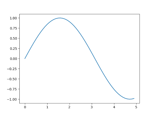
import numpy as np
import matplotlib.pyplot as plt

x = np.arange(0, 5, 0.1);
y = np.sin(x)
plt.plot(x, y)
3D data in NumPy
NumPy arrays can have arbitrarily many dimensions. Just like you can create a 1D array from a list, and a 2D array from a list of lists, you can create a 3D array from a list of lists of lists, and so on. For example, the following code would create a 3D array:
a = np.array([
    [['A1a', 'A1b', 'A1c'], ['A2a', 'A2b', 'A2c']],
    [['B1a', 'B1b', 'B1c'], ['B2a', 'B2b', 'B2c']]
])
3D data in Pandas
Pandas has a data structure called a Panel, which is similar to a DataFrame or a Series, but for 3D data. If you would like, you can learn more about Panels here.