深度学习基础 [课程]
Deep Learning Foundations [Course]

Udacity course link: https://www.udacity.com/course/deep-learning-nanodegree--nd101
Applying deep learning
Resource
- Grokking Deep Learning by Andrew Trask. Use our exclusive discount code traskud17 for 40% off. This provides a very gentle introduction to Deep Learning and covers the intuition more than the theory.
- Neural Networks And Deep Learning by Michael Nielsen. This book is more rigorous than Grokking Deep Learning and includes a lot of fun, interactive visualizations to play with.
- The Deep Learning Textbook from Ian Goodfellow, Yoshua Bengio, and Aaron Courville. This online book has lot of material and is the most rigorous of the three books suggested.
- 10 minutes to Pandas
- Scikit-Learn official tutorial
- Matplotlib official tutorial
Linear regression
Conduct linear regression using scikit-learn:
>>> from sklearn.linear_model import LinearRegression
>>> model = LinearRegression()
>>> model.fit(x_values, y_values)
>>> print(model.predict([ [127], [248] ]))
[[ 438.94308857, 127.14839521]]
The model returned an array of predictions, one prediction for each input array. The first input, [127], got a prediction of 438.94308857. The seconds input, [248], got a prediction of 127.14839521. The reason for predicting on an array like [127] and not just 127, is because you can have a model that makes a prediction using multiple features.
For Pandas DataFrames, single square brackets return a Pandas Series, while double square brackets return a DataFrame. Example:
import pandas as pd
from sklearn.linear_model import LinearRegression

# Load the data
bmi_life_data = pd.read_csv("bmi_and_life_expectancy.csv")

# Fit the model and Assign it to bmi_life_model
bmi_life_model = LinearRegression()
bmi_life_model.fit(bmi_life_data[['BMI']],   # Must be double brackets
    bmi_life_data[['Life expectancy']])      # [col1, col2, ...] as a list

# Predict life expectancy for a BMI value of 21.07931
laos_life_exp = bmi_life_model.predict(21.07931)
Multivariable linear regression works the same.
Warnings:
- Linear Regression Works Best When the Data is Linear
- Linear Regression is Sensitive to Outliers
Data in NumPy
>>> import numpy as np
>>> s = np.array(5)
>>> s.shape
()   # scalar: 0 dimension

>>> v = np.array([1,2,3])
>>> v.shape
(3,)   # vector: 1 dimension
>>> v[1]
2

>>> m = np.array([[1,2,3], [4,5,6], [7,8,9]])
>>> m.shape
(3, 3)   # matrix: 2 dimension
>>> m[1][2]
6

>>> t = np.array([[[[1],[2]],[[3],[4]],[[5],[6]]],[[[7],[8]],\
    [[9],[10]],[[11],[12]]],[[[13],[14]],[[15],[16]],[[17],[17]]]])
>>> t.shape
(3, 3, 2, 1)
>>> t[2][1][1][0]
16

>>> v = np.array([1,2,3,4])
>>> v.shape
(4,)
>>> x = v.reshape(1,4)   # reshape

>>> x = v[None, :]   # add a new dimension of size 1 for the associated axis
Element-wise Multiplication
You saw some element-wise multiplication already. You accomplish that with the multiply function or the * operator. Just to revisit, it would look like this:
m = np.array([[1,2,3],[4,5,6]])
m
# displays the following result:
# array([[1, 2, 3],
#        [4, 5, 6]])

n = m * 0.25
n
# displays the following result:
# array([[ 0.25,  0.5 ,  0.75],
#        [ 1.  ,  1.25,  1.5 ]])

m * n
# displays the following result:
# array([[ 0.25,  1.  ,  2.25],
#        [ 4.  ,  6.25,  9.  ]])

np.multiply(m, n)   # equivalent to m * n
# displays the following result:
# array([[ 0.25,  1.  ,  2.25],
#        [ 4.  ,  6.25,  9.  ]])
Matrix Product
To find the matrix product, you use NumPy’s matmul function.
If you have compatible shapes, then it’s as simple as this:
a = np.array([[1,2,3,4],[5,6,7,8]])
a
# displays the following result:
# array([[1, 2, 3, 4],
#        [5, 6, 7, 8]])
a.shape
# displays the following result:
# (2, 4)

b = np.array([[1,2,3],[4,5,6],[7,8,9],[10,11,12]])
b
# displays the following result:
# array([[ 1,  2,  3],
#        [ 4,  5,  6],
#        [ 7,  8,  9],
#        [10, 11, 12]])
b.shape
# displays the following result:
# (4, 3)

c = np.matmul(a, b)
c
# displays the following result:
# array([[ 70,  80,  90],
#        [158, 184, 210]])
c.shape
# displays the following result:
# (2, 3)
If your matrices have incompatible shapes, you’ll get an error, like the following:
np.matmul(b, a)
# displays the following error:
# ValueError: shapes (4,3) and (2,4) not aligned: 3 (dim 1) != 2 (dim 0)
NumPy’s dot function
You may sometimes see NumPy’s dot function in places where you would expect a matmul. It turns out that the results of dot and matmul are the same if the matrices are two dimensional.
So these two results are equivalent:
a = np.array([[1,2],[3,4]])
a
# displays the following result:
# array([[1, 2],
#        [3, 4]])

np.dot(a,a)
# displays the following result:
# array([[ 7, 10],
#        [15, 22]])

a.dot(a)  # you can call `dot` directly on the `ndarray`
# displays the following result:
# array([[ 7, 10],
#        [15, 22]])

np.matmul(a,a)
# array([[ 7, 10],
#        [15, 22]])
While these functions return the same results for two dimensional data, you should be careful about which you choose when working with other data shapes. You can read more about the differences, and find links to other NumPy functions, in the matmul and dot documentation.
Transpose
Getting the transpose of a matrix is really easy in NumPy. Simply access its T attribute. There is also a transpose() function which returns the same thing, but you’ll rarely see that used anywhere because typing T is so much easier. :)
For example:
m = np.array([[1,2,3,4], [5,6,7,8], [9,10,11,12]])
m
# displays the following result:
# array([[ 1,  2,  3,  4],
#        [ 5,  6,  7,  8],
#        [ 9, 10, 11, 12]])

m.T
# displays the following result:
# array([[ 1,  5,  9],
#        [ 2,  6, 10],
#        [ 3,  7, 11],
#        [ 4,  8, 12]])
NumPy does this without actually moving any data in memory - it simply changes the way it indexes the original matrix - so it’s quite efficient.
However, that also means you need to be careful with how you modify objects, because they are sharing the same data. For example, with the same matrix m from above, let’s make a new variable m_t that stores m’s transpose. Then look what happens if we modify a value in m_t:
m_t = m.T
m_t[3][1] = 200
m_t
# displays the following result:
# array([[ 1,   5, 9],
#        [ 2,   6, 10],
#        [ 3,   7, 11],
#        [ 4, 200, 12]])

m
# displays the following result:
# array([[ 1,  2,  3,   4],
#        [ 5,  6,  7, 200],
#        [ 9, 10, 11,  12]])
Notice how it modified both the transpose and the original matrix, too! That’s because they are sharing the same copy of data. So remember to consider the transpose just as a different view of your matrix, rather than a different matrix entirely.
Create a 2 dimensional array from a one dimensional list: np.reshape([2,4,6,1],((-1,2)))
Gradient descent
One weight update can be calculated as:
\[\Delta{w_i} = \eta \delta{x_i} \]with the error term \(\delta\) as
\[\delta = ( y − \hat{y} ) f'(h) = ( y − \hat{y} ) f'(\sum{w_i x_i})\]Remember, in the above equation \(\eta\) is the learning rate, \((y - \hat{y})\) is the output error, and \(f’(h)\) refers to the derivative of the activation function, \(f(h)\) . We’ll call that derivative the output gradient.
The derivative of sigmoid function has a nice feature:
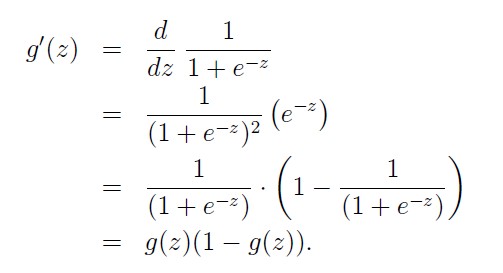
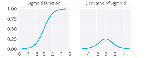
Now I’ll write this out in code for the case of only one output unit. We’ll also be using the sigmoid as the activation function \(f(h)\) .
# Defining the sigmoid function for activations
def sigmoid(x):
    return 1/(1+np.exp(-x))

# Derivative of the sigmoid function
def sigmoid_prime(x):
    return sigmoid(x) * (1 - sigmoid(x))

# Input data
x = np.array([0.1, 0.3])
# Target
y = 0.2
# Input to output weights
weights = np.array([-0.8, 0.5])

# The learning rate, eta in the weight step equation
learnrate = 0.5

# the linear combination performed by the node (h in f(h) and f'(h))
h = x[0]*weights[0] + x[1]*weights[1]
# or h = np.dot(x, weights)

# The neural network output (y-hat)
nn_output = sigmoid(h)

# output error (y - y-hat)
error = y - nn_output

# output gradient (f'(h))
output_grad = sigmoid_prime(h)

# error term (lowercase delta)
error_term = error * output_grad

# Gradient descent step
del_w = [ learnrate * error_term * x[0],
          learnrate * error_term * x[1]]
# or del_w = learnrate * error_term * x
Batch learning:
import numpy as np
from data_prep import features, targets, features_test, targets_test

def sigmoid(x):
    """
    Calculate sigmoid
    """
    return 1 / (1 + np.exp(-x))

# Use to same seed to make debugging easier
np.random.seed(42)

n_records, n_features = features.shape
last_loss = None

# Initialize weights
weights = np.random.normal(scale=1 / n_features**.5, size=n_features)

# Neural Network hyperparameters
epochs = 1000
learnrate = 0.5

for e in range(epochs):
    del_w = np.zeros(weights.shape)
    for x, y in zip(features.values, targets):
        # Loop through all records, x is the input, y is the target

        # Activation of the output unit
        #   Notice we multiply the inputs and the weights here
        #   rather than storing h as a separate variable
        output = sigmoid(np.dot(x, weights))

        # The error, the target minus the network output
        error = y - output

        # The error term
        #   Notice we calulate f'(h) here instead of defining a separate
        #   sigmoid_prime function. This just makes it faster because we
        #   can re-use the result of the sigmoid function stored in
        #   the output variable
        error_term = error * output * (1 - output)

        # The gradient descent step, the error times the gradient times the inputs
        del_w += error_term * x

    # Update the weights here. The learning rate times the
    # change in weights, divided by the number of records to average
    weights += learnrate * del_w / n_records

    # Printing out the mean square error on the training set
    if e % (epochs / 10) == 0:
        out = sigmoid(np.dot(features, weights))
        loss = np.mean((out - targets) ** 2)
        if last_loss and last_loss < loss:
            print("Train loss: ", loss, "  WARNING - Loss Increasing")
        else:
            print("Train loss: ", loss)
        last_loss = loss

# Calculate accuracy on test data
tes_out = sigmoid(np.dot(features_test, weights))
predictions = tes_out > 0.5
accuracy = np.mean(predictions == targets_test)
print("Prediction accuracy: {:.3f}".format(accuracy))

'''
Train loss:  0.2627609385
Train loss:  0.209286194093
Train loss:  0.200842929081
Train loss:  0.198621564755
Train loss:  0.197798513967
Train loss:  0.197425779122
Train loss:  0.197235077462
Train loss:  0.197129456251
Train loss:  0.197067663413
Train loss:  0.197030058018
Prediction accuracy: 0.725
'''
Making a column vector
You see above that sometimes you’ll want a column vector, even though by default Numpy arrays work like row vectors. It’s possible to get the transpose of an array like so arr.T, but for a 1D array, the transpose will return a row vector. Instead, use arr[:,None]` to create a column vector:
print(features)
> array([ 0.49671415, -0.1382643 ,  0.64768854])

print(features.T)
> array([ 0.49671415, -0.1382643 ,  0.64768854])

print(features[:, None])
> array([[ 0.49671415],
       [-0.1382643 ],
       [ 0.64768854]])
Backpropagation
For example, in the output layer, you have errors \(\delta^o_k\) attributed to each output unit \(k\). Then, the error attributed to hidden unit \(j\) is the output errors, scaled by the weights between the output and hidden layers (and the gradient):
\[\delta^h_j = \sum W_{jk} \delta^o_k f'(h_j)\]Then, the gradient descent step is the same as before, just with the new errors:
\[\Delta w_{ij} = \eta \delta^h_j x_i\]where \(w_{ij}\) are the weights between the inputs and hidden layer and \(x_i\) are input unit values. This form holds for however many layers there are. The weight steps are equal to the step size times the output error of the layer times the values of the inputs to that layer
\[\Delta w_{pq} = \eta \delta_{output} V_{in}\]Here, you get the output error, \(\delta_{output}\), by propagating the errors backwards from higher layers. And the input values, \(V_{in}\) are the inputs to the layer, the hidden layer activations to the output unit for example.
import numpy as np


def sigmoid(x):
    """
    Calculate sigmoid
    """
    return 1 / (1 + np.exp(-x))


x = np.array([0.5, 0.1, -0.2])
target = 0.6
learnrate = 0.5

weights_input_hidden = np.array([[0.5, -0.6],
                                 [0.1, -0.2],
                                 [0.1, 0.7]])

weights_hidden_output = np.array([0.1, -0.3])

## Forward pass
hidden_layer_input = np.dot(x, weights_input_hidden)
hidden_layer_output = sigmoid(hidden_layer_input)

output_layer_in = np.dot(hidden_layer_output, weights_hidden_output)
output = sigmoid(output_layer_in)

## Backwards pass
## TODO: Calculate output error
error = target - output

# TODO: Calculate error term for output layer
output_error_term = error * output * (1-output)

# TODO: Calculate error term for hidden layer
hidden_error_term = np.dot(weights_hidden_output, output_error_term) * \
                    hidden_layer_output * (1-hidden_layer_output)

# TODO: Calculate change in weights for hidden layer to output layer
delta_w_h_o = learnrate * output_error_term * hidden_layer_output

# TODO: Calculate change in weights for input layer to hidden layer
delta_w_i_h = learnrate * hidden_error_term * x[:, None]

print('Change in weights for hidden layer to output layer:')
print(delta_w_h_o)
print('Change in weights for input layer to hidden layer:')
print(delta_w_i_h)

'''
Change in weights for hidden layer to output layer:
[ 0.00804047  0.00555918]
Change in weights for input layer to hidden layer:
[[  1.77005547e-04  -5.11178506e-04]
 [  3.54011093e-05  -1.02235701e-04]
 [ -7.08022187e-05   2.04471402e-04]]
'''
Backpropagation with batch Learning
Now we’ve seen that the error term for the output layer is
\[\delta_k = (y_k - \hat{y_k}) f'(a_k)\]and the error term for the hidden layer is
\[\delta_j = \sum [w_{jk} \delta_k] f'(h_j)\]For now we’ll only consider a simple network with one hidden layer and one output unit. Here’s the general algorithm for updating the weights with backpropagation:
-
Set the weight steps for each layer to zero
-
The input to hidden weights \(\Delta w_{ij} = 0\)
-
The hidden to output weights \(\Delta W_j = 0\)
-
-
For each record in the training data:
-
Make a forward pass through the network, calculating the output \(\hat{y}\)
-
Calculate the error gradient in the output unit, \(\delta^o = (y - \hat{y}) f’(z)\) where \(z = \sum W_j a_j\), the input to the output unit.
-
Propagate the errors to the hidden layer \(\delta^h_j = \delta^o W_j f’(h_j)\)
-
Update the weight steps,
-
\(\Delta W_j = \Delta W_j + \delta^o a_j\)
-
\(\Delta w_{ij} = \Delta w_{ij} + \delta^h_j a_i\)
-
-
-
Update the weights, where \(\eta\) is the learning rate and \(m\) is the number of records:
-
\(W_j = W_j + \eta \Delta W_j / m\)
-
\(w_{ij} = w_{ij} + \eta \Delta w_{ij} / m\)
-
-
Repeat for \(e\) epochs.
import numpy as np
from data_prep import features, targets, features_test, targets_test

np.random.seed(21)

def sigmoid(x):
    """
    Calculate sigmoid
    """
    return 1 / (1 + np.exp(-x))


# Hyperparameters
n_hidden = 2  # number of hidden units
epochs = 900
learnrate = 0.005

n_records, n_features = features.shape
last_loss = None
# Initialize weights
weights_input_hidden = np.random.normal(scale=1 / n_features ** .5,
                                        size=(n_features, n_hidden))
weights_hidden_output = np.random.normal(scale=1 / n_features ** .5,
                                         size=n_hidden)

for e in range(epochs):
    del_w_input_hidden = np.zeros(weights_input_hidden.shape)
    del_w_hidden_output = np.zeros(weights_hidden_output.shape)
    for x, y in zip(features.values, targets):
        ## Forward pass ##
        # TODO: Calculate the output
        hidden_input = np.dot(x, weights_input_hidden)
        hidden_output = sigmoid(hidden_input)
        output = sigmoid(np.dot(hidden_output, weights_hidden_output))

        ## Backward pass ##
        # TODO: Calculate the network's prediction error
        error = y - output

        # TODO: Calculate error term for the output unit
        output_error_term = error * output * (1-output)

        ## propagate errors to hidden layer

        # TODO: Calculate the hidden layer's contribution to the error
        hidden_error = np.dot(output_error_term, weights_hidden_output)

        # TODO: Calculate the error term for the hidden layer
        hidden_error_term = hidden_error * hidden_output * (1-hidden_output)

        # TODO: Update the change in weights
        del_w_hidden_output += hidden_output * output_error_term
        del_w_input_hidden += x[:, None] * hidden_error_term

    # TODO: Update weights
    weights_input_hidden += learnrate * del_w_input_hidden / n_records
    weights_hidden_output += learnrate * del_w_hidden_output / n_records

    # Printing out the mean square error on the training set
    if e % (epochs / 10) == 0:
        hidden_output = sigmoid(np.dot(x, weights_input_hidden))
        out = sigmoid(np.dot(hidden_output,
                             weights_hidden_output))
        loss = np.mean((out - targets) ** 2)

        if last_loss and last_loss < loss:
            print("Train loss: ", loss, "  WARNING - Loss Increasing")
        else:
            print("Train loss: ", loss)
        last_loss = loss

# Calculate accuracy on test data
hidden = sigmoid(np.dot(features_test, weights_input_hidden))
out = sigmoid(np.dot(hidden, weights_hidden_output))
predictions = out > 0.5
accuracy = np.mean(predictions == targets_test)
print("Prediction accuracy: {:.3f}".format(accuracy))

'''
Train loss:  0.251357252426
Train loss:  0.249965407188
Train loss:  0.248620052189
Train loss:  0.247319932172
Train loss:  0.246063804656
Train loss:  0.244850441793
Train loss:  0.243678632019
Train loss:  0.242547181518
Train loss:  0.241454915502
Train loss:  0.240400679325
Prediction accuracy: 0.725

Nice job!  That's right!
'''